Statistics in R

Author

Install libraries (only once)

# install.packages("tidyverse")
# install.packages("viridis")
# install.packages("broom")

# load libraries
library(tidyverse)
library(viridis)
library(broom)

2020-03-20 Statistics in R

We’ve finally gotten to what R was meant for! Statistics!

T-test

One sample t-ttest

For testing the mean of some continuous data against a known mean.

iris$Sepal.Length

  [1] 5.1 4.9 4.7 4.6 5.0 5.4 4.6 5.0 4.4 4.9 5.4 4.8 4.8 4.3 5.8 5.7 5.4 5.1
 [19] 5.7 5.1 5.4 5.1 4.6 5.1 4.8 5.0 5.0 5.2 5.2 4.7 4.8 5.4 5.2 5.5 4.9 5.0
 [37] 5.5 4.9 4.4 5.1 5.0 4.5 4.4 5.0 5.1 4.8 5.1 4.6 5.3 5.0 7.0 6.4 6.9 5.5
 [55] 6.5 5.7 6.3 4.9 6.6 5.2 5.0 5.9 6.0 6.1 5.6 6.7 5.6 5.8 6.2 5.6 5.9 6.1
 [73] 6.3 6.1 6.4 6.6 6.8 6.7 6.0 5.7 5.5 5.5 5.8 6.0 5.4 6.0 6.7 6.3 5.6 5.5
 [91] 5.5 6.1 5.8 5.0 5.6 5.7 5.7 6.2 5.1 5.7 6.3 5.8 7.1 6.3 6.5 7.6 4.9 7.3
[109] 6.7 7.2 6.5 6.4 6.8 5.7 5.8 6.4 6.5 7.7 7.7 6.0 6.9 5.6 7.7 6.3 6.7 7.2
[127] 6.2 6.1 6.4 7.2 7.4 7.9 6.4 6.3 6.1 7.7 6.3 6.4 6.0 6.9 6.7 6.9 5.8 6.8
[145] 6.7 6.7 6.3 6.5 6.2 5.9

ggplot(iris, aes(x =0 ,y=Sepal.Length)) +
  geom_boxplot()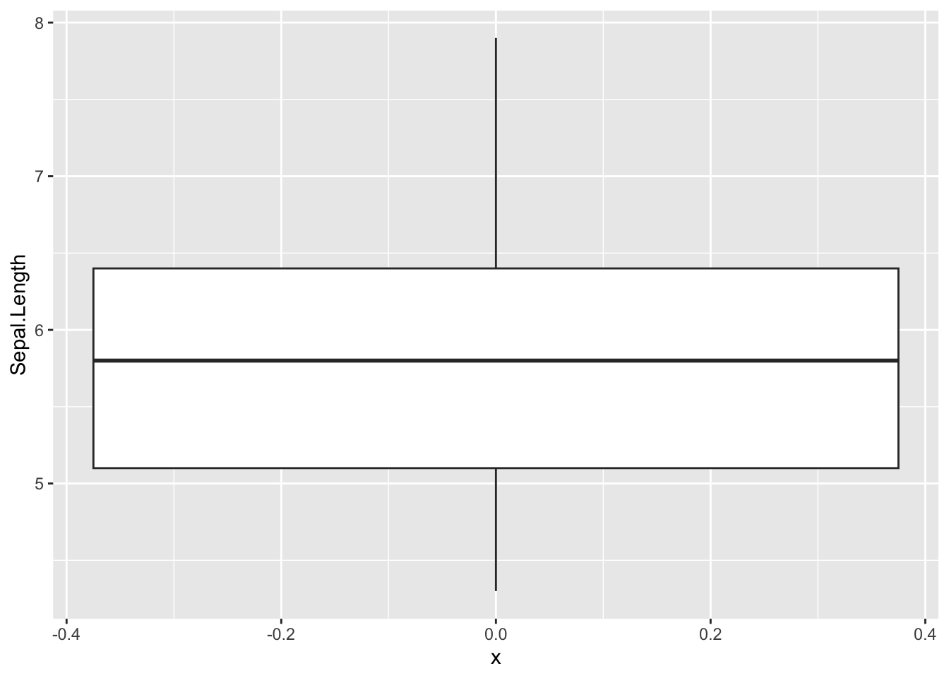

iris$Sepal.Length

  [1] 5.1 4.9 4.7 4.6 5.0 5.4 4.6 5.0 4.4 4.9 5.4 4.8 4.8 4.3 5.8 5.7 5.4 5.1
 [19] 5.7 5.1 5.4 5.1 4.6 5.1 4.8 5.0 5.0 5.2 5.2 4.7 4.8 5.4 5.2 5.5 4.9 5.0
 [37] 5.5 4.9 4.4 5.1 5.0 4.5 4.4 5.0 5.1 4.8 5.1 4.6 5.3 5.0 7.0 6.4 6.9 5.5
 [55] 6.5 5.7 6.3 4.9 6.6 5.2 5.0 5.9 6.0 6.1 5.6 6.7 5.6 5.8 6.2 5.6 5.9 6.1
 [73] 6.3 6.1 6.4 6.6 6.8 6.7 6.0 5.7 5.5 5.5 5.8 6.0 5.4 6.0 6.7 6.3 5.6 5.5
 [91] 5.5 6.1 5.8 5.0 5.6 5.7 5.7 6.2 5.1 5.7 6.3 5.8 7.1 6.3 6.5 7.6 4.9 7.3
[109] 6.7 7.2 6.5 6.4 6.8 5.7 5.8 6.4 6.5 7.7 7.7 6.0 6.9 5.6 7.7 6.3 6.7 7.2
[127] 6.2 6.1 6.4 7.2 7.4 7.9 6.4 6.3 6.1 7.7 6.3 6.4 6.0 6.9 6.7 6.9 5.8 6.8
[145] 6.7 6.7 6.3 6.5 6.2 5.9

mean(iris$Sepal.Length)

[1] 5.843333

### significant result
t.test(iris$Sepal.Length, mu = 10)


    One Sample t-test

data:  iris$Sepal.Length
t = -61.479, df = 149, p-value < 2.2e-16
alternative hypothesis: true mean is not equal to 10
95 percent confidence interval:
 5.709732 5.976934
sample estimates:
mean of x 
 5.843333

### non-significant result
t.test(iris$Sepal.Length, mu = 5.8)


    One Sample t-test

data:  iris$Sepal.Length
t = 0.64092, df = 149, p-value = 0.5226
alternative hypothesis: true mean is not equal to 5.8
95 percent confidence interval:
 5.709732 5.976934
sample estimates:
mean of x 
 5.843333

Lets vizualize what we are testing

ggplot(iris, aes(x =0 , y=Sepal.Length)) +
  geom_boxplot() +
  geom_jitter(width = 0.1) +
  geom_hline(yintercept = 10, color='red', linewidth = 2, linetype = 'dashed')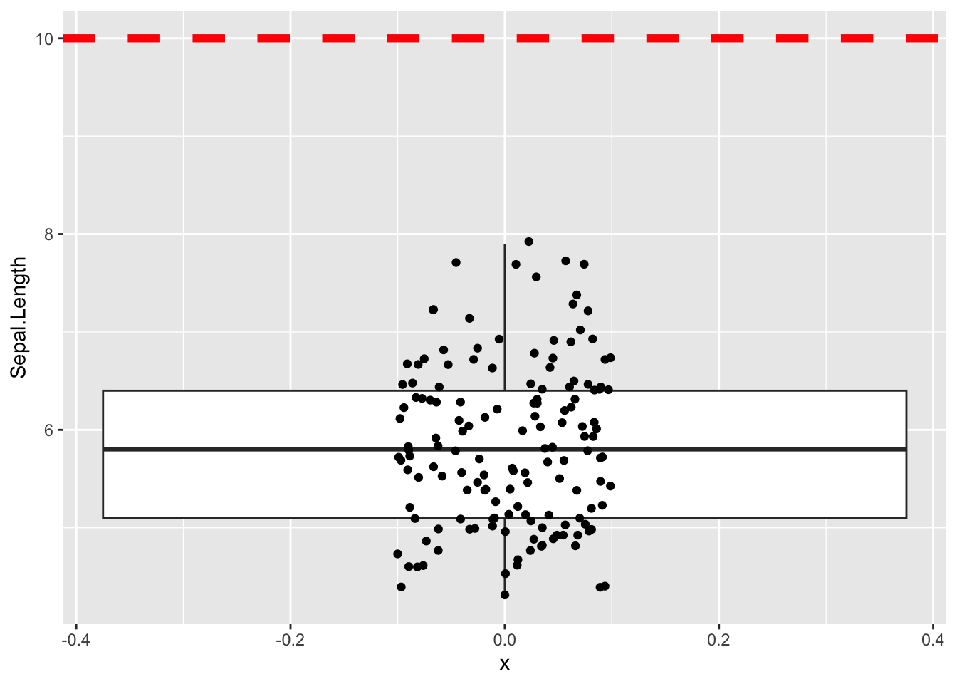

Using broom functions to tidy up t.test()

t.test(iris$Sepal.Length, mu = 5)


    One Sample t-test

data:  iris$Sepal.Length
t = 12.473, df = 149, p-value < 2.2e-16
alternative hypothesis: true mean is not equal to 5
95 percent confidence interval:
 5.709732 5.976934
sample estimates:
mean of x 
 5.843333

# tidy()
# Gets the result of the test
t.test(iris$Sepal.Length, mu = 5) %>% tidy()

# A tibble: 1 × 8
  estimate statistic  p.value parameter conf.low conf.high method    alternative
     <dbl>     <dbl>    <dbl>     <dbl>    <dbl>     <dbl> <chr>     <chr>      
1     5.84      12.5 6.67e-25       149     5.71      5.98 One Samp… two.sided

# glance()
# Gets the model parameters; frequently some of the columns will be the same as
# the ones you get with tidy(). With t.test() tidy() and glance() actually 
# return exactly the same results.
t.test(iris$Sepal.Length, mu = 5) %>% glance()

# A tibble: 1 × 8
  estimate statistic  p.value parameter conf.low conf.high method    alternative
     <dbl>     <dbl>    <dbl>     <dbl>    <dbl>     <dbl> <chr>     <chr>      
1     5.84      12.5 6.67e-25       149     5.71      5.98 One Samp… two.sided

Two sample t-test

For testing the difference in means between two groups

unpaired

This is the standard t-test that you should use by default

# How to pipe into t.test
iris %>% 
# filter out one species, because we can only test two groups
  filter(Species != 'setosa') %>%
# Syntax is numeric variable ~ grouping variable
# Need to use . when piping; this tells t.test() that the table is being piped in
  t.test(Sepal.Length ~ Species, data = .)


    Welch Two Sample t-test

data:  Sepal.Length by Species
t = -5.6292, df = 94.025, p-value = 1.866e-07
alternative hypothesis: true difference in means between group versicolor and group virginica is not equal to 0
95 percent confidence interval:
 -0.8819731 -0.4220269
sample estimates:
mean in group versicolor  mean in group virginica 
                   5.936                    6.588

### with tidy()
iris %>% 
  filter(Species != 'setosa') %>%
  t.test(Sepal.Length ~ Species, data = .) %>%
  tidy()

# A tibble: 1 × 10
  estimate estimate1 estimate2 statistic    p.value parameter conf.low conf.high
     <dbl>     <dbl>     <dbl>     <dbl>      <dbl>     <dbl>    <dbl>     <dbl>
1   -0.652      5.94      6.59     -5.63    1.87e-7      94.0   -0.882    -0.422
# ℹ 2 more variables: method <chr>, alternative <chr>

Lets vizualize what we are testing

iris %>% 
  filter(Species != 'setosa') %>% 
ggplot(aes(x = Species , y=Sepal.Length, fill = Species)) +
  geom_boxplot() +
  geom_jitter(width = 0.1)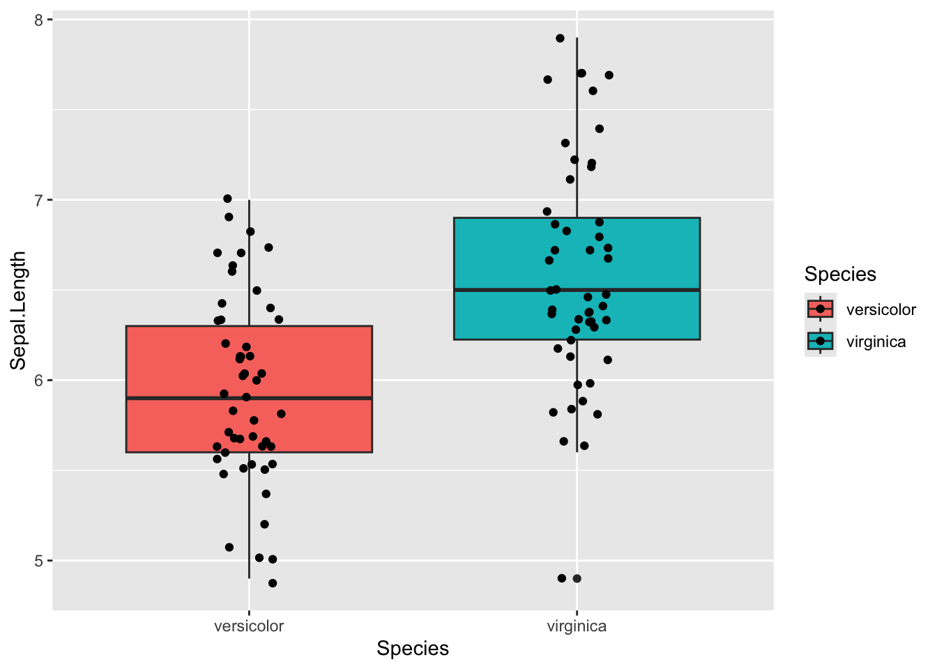

what going under hood of R test

vector_1 <- iris %>% 
  filter(Species=="versicolor") %>% 
  select(Sepal.Length)

vector_2 <- iris %>% 
  filter(Species=="virginica") %>% 
  select(Sepal.Length)

vector_1

   Sepal.Length
1           7.0
2           6.4
3           6.9
4           5.5
5           6.5
6           5.7
7           6.3
8           4.9
9           6.6
10          5.2
11          5.0
12          5.9
13          6.0
14          6.1
15          5.6
16          6.7
17          5.6
18          5.8
19          6.2
20          5.6
21          5.9
22          6.1
23          6.3
24          6.1
25          6.4
26          6.6
27          6.8
28          6.7
29          6.0
30          5.7
31          5.5
32          5.5
33          5.8
34          6.0
35          5.4
36          6.0
37          6.7
38          6.3
39          5.6
40          5.5
41          5.5
42          6.1
43          5.8
44          5.0
45          5.6
46          5.7
47          5.7
48          6.2
49          5.1
50          5.7

vector_2

   Sepal.Length
1           6.3
2           5.8
3           7.1
4           6.3
5           6.5
6           7.6
7           4.9
8           7.3
9           6.7
10          7.2
11          6.5
12          6.4
13          6.8
14          5.7
15          5.8
16          6.4
17          6.5
18          7.7
19          7.7
20          6.0
21          6.9
22          5.6
23          7.7
24          6.3
25          6.7
26          7.2
27          6.2
28          6.1
29          6.4
30          7.2
31          7.4
32          7.9
33          6.4
34          6.3
35          6.1
36          7.7
37          6.3
38          6.4
39          6.0
40          6.9
41          6.7
42          6.9
43          5.8
44          6.8
45          6.7
46          6.7
47          6.3
48          6.5
49          6.2
50          5.9

t.test(vector_1, vector_2)


    Welch Two Sample t-test

data:  vector_1 and vector_2
t = -5.6292, df = 94.025, p-value = 1.866e-07
alternative hypothesis: true difference in means is not equal to 0
95 percent confidence interval:
 -0.8819731 -0.4220269
sample estimates:
mean of x mean of y 
    5.936     6.588

t.test(Sepal.Length ~ Species, data = filter(iris, Species != 'setosa'))


    Welch Two Sample t-test

data:  Sepal.Length by Species
t = -5.6292, df = 94.025, p-value = 1.866e-07
alternative hypothesis: true difference in means between group versicolor and group virginica is not equal to 0
95 percent confidence interval:
 -0.8819731 -0.4220269
sample estimates:
mean in group versicolor  mean in group virginica 
                   5.936                    6.588

even more underhood

data are splitted into 2 vectors

# iris$Sepal.Length
# 
# iris$Species == "versicolor"
# 
# iris[iris$Species=="versicolor",]

iris[iris$Species=="versicolor",]$Sepal.Length

 [1] 7.0 6.4 6.9 5.5 6.5 5.7 6.3 4.9 6.6 5.2 5.0 5.9 6.0 6.1 5.6 6.7 5.6 5.8 6.2
[20] 5.6 5.9 6.1 6.3 6.1 6.4 6.6 6.8 6.7 6.0 5.7 5.5 5.5 5.8 6.0 5.4 6.0 6.7 6.3
[39] 5.6 5.5 5.5 6.1 5.8 5.0 5.6 5.7 5.7 6.2 5.1 5.7

iris[iris$Species=="virginica",]$Sepal.Length

 [1] 6.3 5.8 7.1 6.3 6.5 7.6 4.9 7.3 6.7 7.2 6.5 6.4 6.8 5.7 5.8 6.4 6.5 7.7 7.7
[20] 6.0 6.9 5.6 7.7 6.3 6.7 7.2 6.2 6.1 6.4 7.2 7.4 7.9 6.4 6.3 6.1 7.7 6.3 6.4
[39] 6.0 6.9 6.7 6.9 5.8 6.8 6.7 6.7 6.3 6.5 6.2 5.9

t-test is run on vectoers 2 vectors

vector_1 <-  iris[iris$Species=="versicolor",]$Sepal.Length

vector_2 <-  iris[iris$Species=="virginica",]$Sepal.Length

vector_1

 [1] 7.0 6.4 6.9 5.5 6.5 5.7 6.3 4.9 6.6 5.2 5.0 5.9 6.0 6.1 5.6 6.7 5.6 5.8 6.2
[20] 5.6 5.9 6.1 6.3 6.1 6.4 6.6 6.8 6.7 6.0 5.7 5.5 5.5 5.8 6.0 5.4 6.0 6.7 6.3
[39] 5.6 5.5 5.5 6.1 5.8 5.0 5.6 5.7 5.7 6.2 5.1 5.7

vector_2

 [1] 6.3 5.8 7.1 6.3 6.5 7.6 4.9 7.3 6.7 7.2 6.5 6.4 6.8 5.7 5.8 6.4 6.5 7.7 7.7
[20] 6.0 6.9 5.6 7.7 6.3 6.7 7.2 6.2 6.1 6.4 7.2 7.4 7.9 6.4 6.3 6.1 7.7 6.3 6.4
[39] 6.0 6.9 6.7 6.9 5.8 6.8 6.7 6.7 6.3 6.5 6.2 5.9

t.test(vector_1, vector_2)


    Welch Two Sample t-test

data:  vector_1 and vector_2
t = -5.6292, df = 94.025, p-value = 1.866e-07
alternative hypothesis: true difference in means is not equal to 0
95 percent confidence interval:
 -0.8819731 -0.4220269
sample estimates:
mean of x mean of y 
    5.936     6.588

Paired T test

You can use a paired t-test when a natural pairing exists between the data, for example individuals before and after treatment with some drugs, student test scores at the beginning of the year vs the end of the year, tumor and normal tissue samples from the same individual. The built-in sleep dataset gives the extra sleep time for a group of individuals treated with two different drugs. The columns contain:

extra = numeric increase in hours of sleep
group = drug given
ID = patient ID

Let’s look at the sleep table first.

sleep %>% 
  ggplot(aes(x = group, y = extra, fill=group)) +
  geom_boxplot() +
  geom_point() +
  geom_line(aes(group = ID))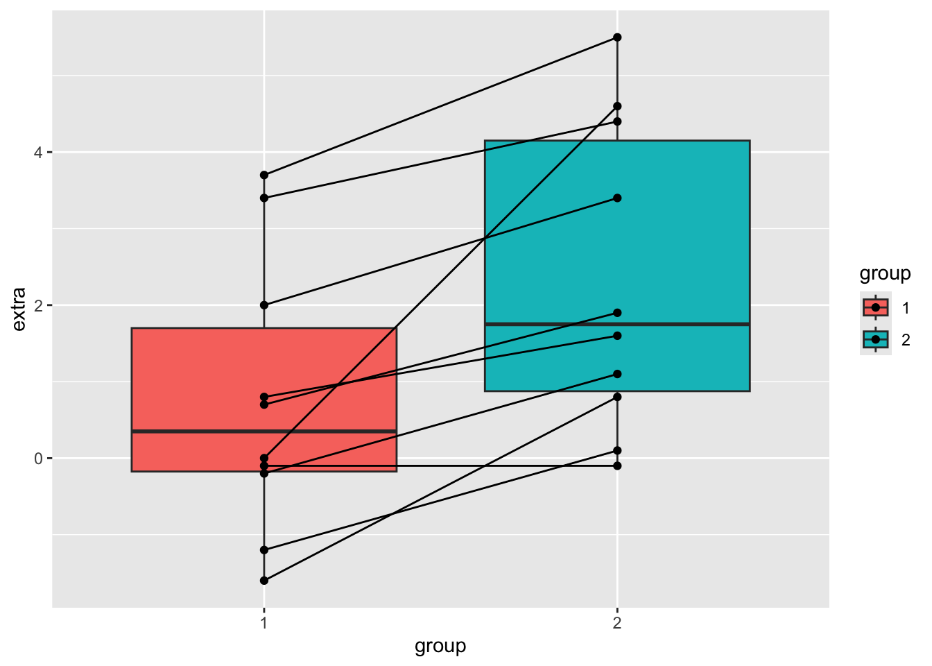

sleep %>% 
  ggplot(aes(x = group, y = extra, colour = ID)) +
  geom_point() +
  geom_line(aes(group = ID))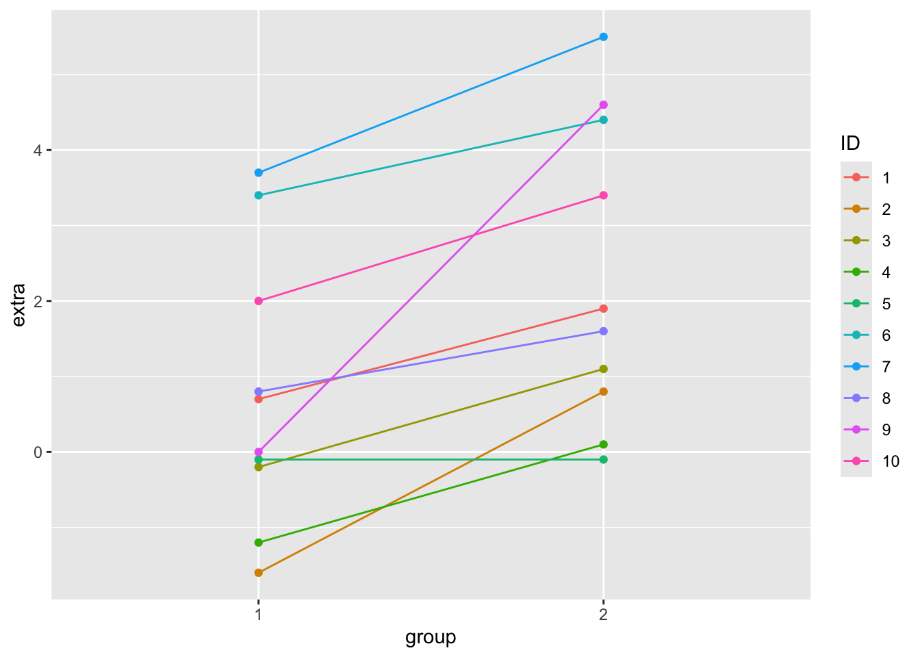

To do a paired t-test, set the argument paired = T. Let’s compare doing a paired and an unpaired t-test on the same data. A paired t-test will always give you a more significant result.

## Paired t-test
## The sleep data is actually paired, so could have been in wide format:
sleep_wide <- pivot_wider(sleep, names_from = group, values_from = "extra") #%>% 

sleep_wide <- sleep_wide %>% 
  rename(time_1 = "1",
         time_2 = "2")

sleep_wide

# A tibble: 10 × 3
   ID    time_1 time_2
   <fct>  <dbl>  <dbl>
 1 1        0.7    1.9
 2 2       -1.6    0.8
 3 3       -0.2    1.1
 4 4       -1.2    0.1
 5 5       -0.1   -0.1
 6 6        3.4    4.4
 7 7        3.7    5.5
 8 8        0.8    1.6
 9 9        0      4.6
10 10       2      3.4

# on long data()
t.test(data = sleep, extra ~ group)


    Welch Two Sample t-test

data:  extra by group
t = -1.8608, df = 17.776, p-value = 0.07939
alternative hypothesis: true difference in means between group 1 and group 2 is not equal to 0
95 percent confidence interval:
 -3.3654832  0.2054832
sample estimates:
mean in group 1 mean in group 2 
           0.75            2.33

# wide data
t.test(sleep_wide$time_1, sleep_wide$time_2)


    Welch Two Sample t-test

data:  sleep_wide$time_1 and sleep_wide$time_2
t = -1.8608, df = 17.776, p-value = 0.07939
alternative hypothesis: true difference in means is not equal to 0
95 percent confidence interval:
 -3.3654832  0.2054832
sample estimates:
mean of x mean of y 
     0.75      2.33

Traditional interface

# wide data
t.test(sleep_wide$time_1, sleep_wide$time_2, paired = TRUE)


    Paired t-test

data:  sleep_wide$time_1 and sleep_wide$time_2
t = -4.0621, df = 9, p-value = 0.002833
alternative hypothesis: true mean difference is not equal to 0
95 percent confidence interval:
 -2.4598858 -0.7001142
sample estimates:
mean difference 
          -1.58

Formula interface

# wide data
t.test(Pair(time_1,time_2) ~ 1, data=sleep_wide)


    Paired t-test

data:  Pair(time_1, time_2)
t = -4.0621, df = 9, p-value = 0.002833
alternative hypothesis: true mean difference is not equal to 0
95 percent confidence interval:
 -2.4598858 -0.7001142
sample estimates:
mean difference 
          -1.58

Chi-square

Do a chi-square test

H0: In Electorate district XYZ the party affiliation is same between genders

# made up data
Elecorate <- data.frame(row.names = c("Democrat", "Independent", "Republican"),
                        male = c(484, 239, 477),
                        female = c(762, 327, 468))

Elecorate

            male female
Democrat     484    762
Independent  239    327
Republican   477    468

Elecorate %>% chisq.test()


    Pearson's Chi-squared test

data:  .
X-squared = 30.07, df = 2, p-value = 2.954e-07

# Results
# H0: rejected
# H1: there is sig difference between gender in party affiliation

What does it look like using the broom functions?

chisq.test(Elecorate) %>% tidy()

# A tibble: 1 × 4
  statistic     p.value parameter method                    
      <dbl>       <dbl>     <int> <chr>                     
1      30.1 0.000000295         2 Pearson's Chi-squared test

chisq.test(Elecorate) %>% glance()

# A tibble: 1 × 4
  statistic     p.value parameter method                    
      <dbl>       <dbl>     <int> <chr>                     
1      30.1 0.000000295         2 Pearson's Chi-squared test

# chisq.test(Elecorate) %>% augment()

Does orientation matter?

Elecorate

            male female
Democrat     484    762
Independent  239    327
Republican   477    468

Elecorate2 <- Elecorate %>% t() %>% as.data.frame()
Elecorate2

       Democrat Independent Republican
male        484         239        477
female      762         327        468

Elecorate2 %>% chisq.test() %>% tidy()

# A tibble: 1 × 4
  statistic     p.value parameter method                    
      <dbl>       <dbl>     <int> <chr>                     
1      30.1 0.000000295         2 Pearson's Chi-squared test

ANOVA

Look at the data

chickwts

   weight      feed
1     179 horsebean
2     160 horsebean
3     136 horsebean
4     227 horsebean
5     217 horsebean
6     168 horsebean
7     108 horsebean
8     124 horsebean
9     143 horsebean
10    140 horsebean
11    309   linseed
12    229   linseed
13    181   linseed
14    141   linseed
15    260   linseed
16    203   linseed
17    148   linseed
18    169   linseed
19    213   linseed
20    257   linseed
21    244   linseed
22    271   linseed
23    243   soybean
24    230   soybean
25    248   soybean
26    327   soybean
27    329   soybean
28    250   soybean
29    193   soybean
30    271   soybean
31    316   soybean
32    267   soybean
33    199   soybean
34    171   soybean
35    158   soybean
36    248   soybean
37    423 sunflower
38    340 sunflower
39    392 sunflower
40    339 sunflower
41    341 sunflower
42    226 sunflower
43    320 sunflower
44    295 sunflower
45    334 sunflower
46    322 sunflower
47    297 sunflower
48    318 sunflower
49    325  meatmeal
50    257  meatmeal
51    303  meatmeal
52    315  meatmeal
53    380  meatmeal
54    153  meatmeal
55    263  meatmeal
56    242  meatmeal
57    206  meatmeal
58    344  meatmeal
59    258  meatmeal
60    368    casein
61    390    casein
62    379    casein
63    260    casein
64    404    casein
65    318    casein
66    352    casein
67    359    casein
68    216    casein
69    222    casein
70    283    casein
71    332    casein

chickwts %>% distinct(feed)

       feed
1 horsebean
2   linseed
3   soybean
4 sunflower
5  meatmeal
6    casein

Do the test

aov(weight ~ feed, data = chickwts)

Call:
   aov(formula = weight ~ feed, data = chickwts)

Terms:
                    feed Residuals
Sum of Squares  231129.2  195556.0
Deg. of Freedom        5        65

Residual standard error: 54.85029
Estimated effects may be unbalanced

aov(weight ~ feed, data = chickwts) %>% summary()

            Df Sum Sq Mean Sq F value   Pr(>F)    
feed         5 231129   46226   15.37 5.94e-10 ***
Residuals   65 195556    3009                     
---
Signif. codes:  0 '***' 0.001 '**' 0.01 '*' 0.05 '.' 0.1 ' ' 1

What does it look like with the different broom functions?

aov(weight ~ feed, data = chickwts) %>% tidy()

# A tibble: 2 × 6
  term         df   sumsq meansq statistic   p.value
  <chr>     <dbl>   <dbl>  <dbl>     <dbl>     <dbl>
1 feed          5 231129. 46226.      15.4  5.94e-10
2 Residuals    65 195556.  3009.      NA   NA

# aov(weight ~ feed, data = chickwts) %>% glance()
# aov(weight ~ feed, data = chickwts) %>% augment()

Post-Hoc Tukey Test

Tukey test explicitly compares all different functions

aov(weight ~ feed, data = chickwts) %>% summary()

            Df Sum Sq Mean Sq F value   Pr(>F)    
feed         5 231129   46226   15.37 5.94e-10 ***
Residuals   65 195556    3009                     
---
Signif. codes:  0 '***' 0.001 '**' 0.01 '*' 0.05 '.' 0.1 ' ' 1

print('---')

[1] "---"

aov(weight ~ feed, data = chickwts) %>% TukeyHSD()

  Tukey multiple comparisons of means
    95% family-wise confidence level

Fit: aov(formula = weight ~ feed, data = chickwts)

$feed
                           diff         lwr       upr     p adj
horsebean-casein    -163.383333 -232.346876 -94.41979 0.0000000
linseed-casein      -104.833333 -170.587491 -39.07918 0.0002100
meatmeal-casein      -46.674242 -113.906207  20.55772 0.3324584
soybean-casein       -77.154762 -140.517054 -13.79247 0.0083653
sunflower-casein       5.333333  -60.420825  71.08749 0.9998902
linseed-horsebean     58.550000  -10.413543 127.51354 0.1413329
meatmeal-horsebean   116.709091   46.335105 187.08308 0.0001062
soybean-horsebean     86.228571   19.541684 152.91546 0.0042167
sunflower-horsebean  168.716667   99.753124 237.68021 0.0000000
meatmeal-linseed      58.159091   -9.072873 125.39106 0.1276965
soybean-linseed       27.678571  -35.683721  91.04086 0.7932853
sunflower-linseed    110.166667   44.412509 175.92082 0.0000884
soybean-meatmeal     -30.480519  -95.375109  34.41407 0.7391356
sunflower-meatmeal    52.007576  -15.224388 119.23954 0.2206962
sunflower-soybean     82.488095   19.125803 145.85039 0.0038845

chickwts %>% 
  ggplot(aes(feed, weight, fill = feed)) +
    geom_boxplot() +
    geom_jitter(width = 0.1)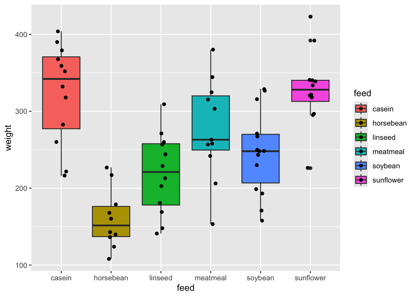

What does it look like with the different `broom` functions?

aov(weight ~ feed, data = chickwts) %>% TukeyHSD() %>% tidy()

# A tibble: 15 × 7
   term  contrast            null.value estimate conf.low conf.high  adj.p.value
   <chr> <chr>                    <dbl>    <dbl>    <dbl>     <dbl>        <dbl>
 1 feed  horsebean-casein             0  -163.    -232.       -94.4 0.0000000307
 2 feed  linseed-casein               0  -105.    -171.       -39.1 0.000210    
 3 feed  meatmeal-casein              0   -46.7   -114.        20.6 0.332       
 4 feed  soybean-casein               0   -77.2   -141.       -13.8 0.00837     
 5 feed  sunflower-casein             0     5.33   -60.4       71.1 1.000       
 6 feed  linseed-horsebean            0    58.6    -10.4      128.  0.141       
 7 feed  meatmeal-horsebean           0   117.      46.3      187.  0.000106    
 8 feed  soybean-horsebean            0    86.2     19.5      153.  0.00422     
 9 feed  sunflower-horsebean          0   169.      99.8      238.  0.0000000122
10 feed  meatmeal-linseed             0    58.2     -9.07     125.  0.128       
11 feed  soybean-linseed              0    27.7    -35.7       91.0 0.793       
12 feed  sunflower-linseed            0   110.      44.4      176.  0.0000884   
13 feed  soybean-meatmeal             0   -30.5    -95.4       34.4 0.739       
14 feed  sunflower-meatmeal           0    52.0    -15.2      119.  0.221       
15 feed  sunflower-soybean            0    82.5     19.1      146.  0.00388

# aov(weight ~ feed, data = chickwts) %>% TukeyHSD() %>% glance()
# aov(weight ~ feed, data = chickwts) %>% TukeyHSD() %>% augment()

anova_chcken_feed <- aov(weight ~ feed, data = chickwts)

anova_chcken_feed %>% TukeyHSD() %>% tidy()

# A tibble: 15 × 7
   term  contrast            null.value estimate conf.low conf.high  adj.p.value
   <chr> <chr>                    <dbl>    <dbl>    <dbl>     <dbl>        <dbl>
 1 feed  horsebean-casein             0  -163.    -232.       -94.4 0.0000000307
 2 feed  linseed-casein               0  -105.    -171.       -39.1 0.000210    
 3 feed  meatmeal-casein              0   -46.7   -114.        20.6 0.332       
 4 feed  soybean-casein               0   -77.2   -141.       -13.8 0.00837     
 5 feed  sunflower-casein             0     5.33   -60.4       71.1 1.000       
 6 feed  linseed-horsebean            0    58.6    -10.4      128.  0.141       
 7 feed  meatmeal-horsebean           0   117.      46.3      187.  0.000106    
 8 feed  soybean-horsebean            0    86.2     19.5      153.  0.00422     
 9 feed  sunflower-horsebean          0   169.      99.8      238.  0.0000000122
10 feed  meatmeal-linseed             0    58.2     -9.07     125.  0.128       
11 feed  soybean-linseed              0    27.7    -35.7       91.0 0.793       
12 feed  sunflower-linseed            0   110.      44.4      176.  0.0000884   
13 feed  soybean-meatmeal             0   -30.5    -95.4       34.4 0.739       
14 feed  sunflower-meatmeal           0    52.0    -15.2      119.  0.221       
15 feed  sunflower-soybean            0    82.5     19.1      146.  0.00388

Linear Model

ggplot(iris, aes(x = Sepal.Width, y = Sepal.Length)) +
  geom_point() +
  geom_smooth(method = 'lm', se = F)

`geom_smooth()` using formula = 'y ~ x'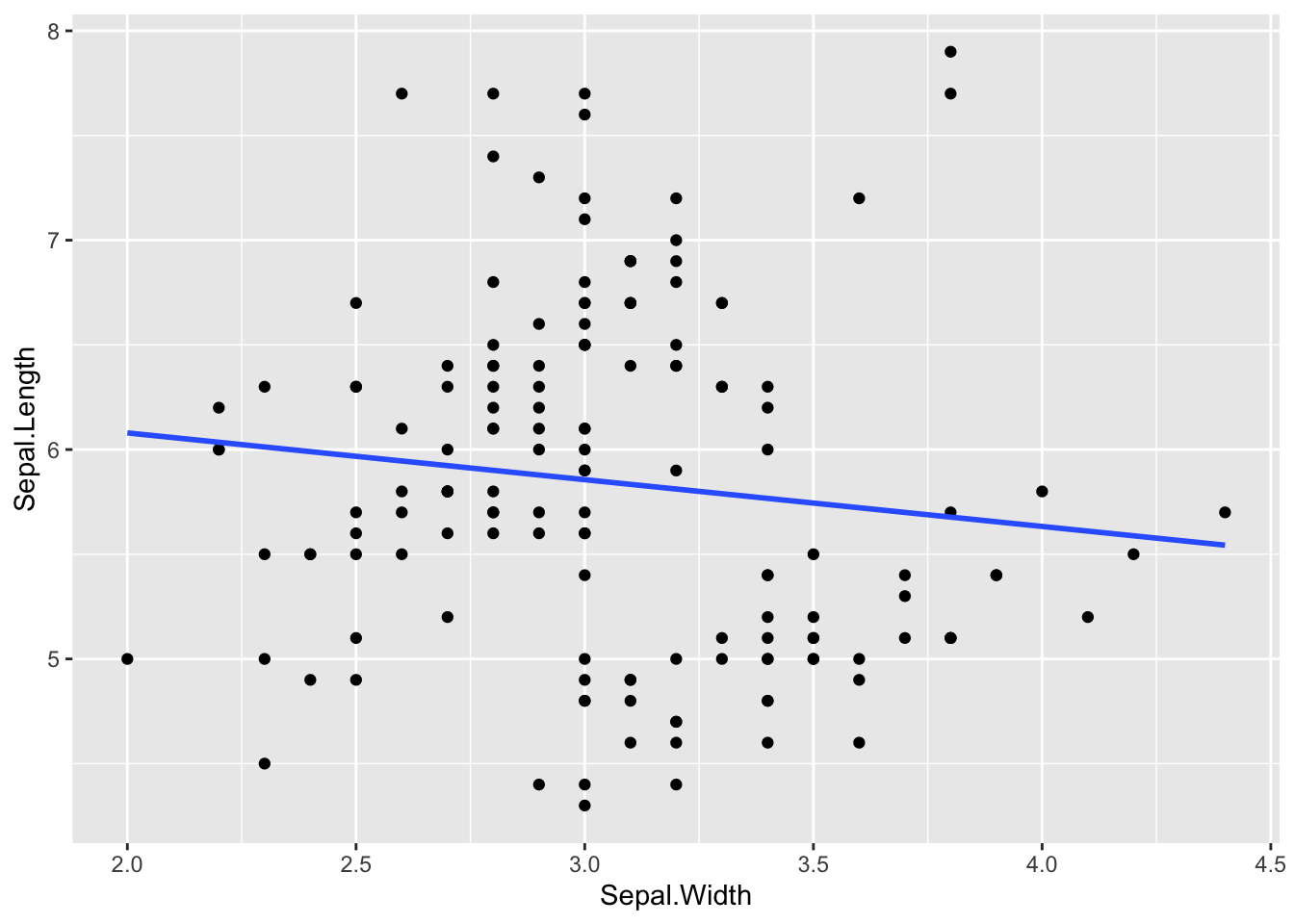

Do the test

### y ~ x
lm(Sepal.Length ~ Sepal.Width, data = iris) %>% summary()


Call:
lm(formula = Sepal.Length ~ Sepal.Width, data = iris)

Residuals:
    Min      1Q  Median      3Q     Max 
-1.5561 -0.6333 -0.1120  0.5579  2.2226 

Coefficients:
            Estimate Std. Error t value Pr(>|t|)    
(Intercept)   6.5262     0.4789   13.63   <2e-16 ***
Sepal.Width  -0.2234     0.1551   -1.44    0.152    
---
Signif. codes:  0 '***' 0.001 '**' 0.01 '*' 0.05 '.' 0.1 ' ' 1

Residual standard error: 0.8251 on 148 degrees of freedom
Multiple R-squared:  0.01382,   Adjusted R-squared:  0.007159 
F-statistic: 2.074 on 1 and 148 DF,  p-value: 0.1519

# lm(Sepal.Width ~ Sepal.Length, data = iris) %>% summary()

What does it look like with the different broom functions?

lm(Sepal.Length ~ Sepal.Width, data = iris) %>% tidy()

# A tibble: 2 × 5
  term        estimate std.error statistic  p.value
  <chr>          <dbl>     <dbl>     <dbl>    <dbl>
1 (Intercept)    6.53      0.479     13.6  6.47e-28
2 Sepal.Width   -0.223     0.155     -1.44 1.52e- 1

# lm(Sepal.Length ~ Sepal.Width, data = iris) %>% glance()
# lm(Sepal.Length ~ Sepal.Width, data = iris) %>% augment(iris)

linear regression when accounted for Species as covariet

ggplot(iris, aes(x = Sepal.Width, y = Sepal.Length, colour = Species)) +
  geom_point() +
  geom_smooth(method = 'lm', se = F)

`geom_smooth()` using formula = 'y ~ x'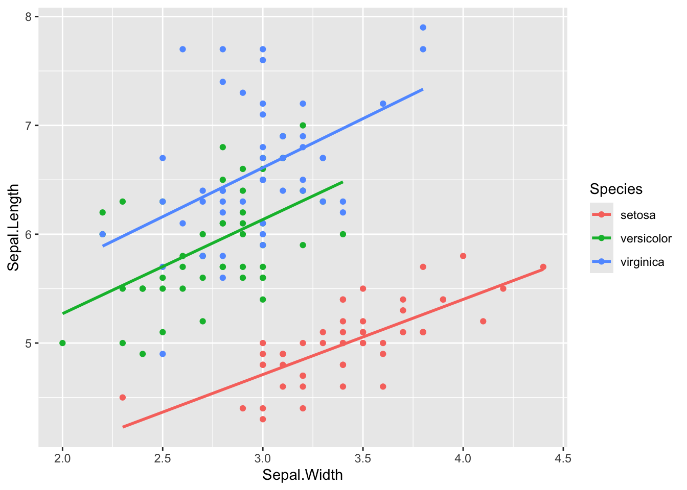

Do the test

### y ~ x
lm(Sepal.Length ~ Sepal.Width + Species, data = iris) %>% summary()


Call:
lm(formula = Sepal.Length ~ Sepal.Width + Species, data = iris)

Residuals:
     Min       1Q   Median       3Q      Max 
-1.30711 -0.25713 -0.05325  0.19542  1.41253 

Coefficients:
                  Estimate Std. Error t value Pr(>|t|)    
(Intercept)         2.2514     0.3698   6.089 9.57e-09 ***
Sepal.Width         0.8036     0.1063   7.557 4.19e-12 ***
Speciesversicolor   1.4587     0.1121  13.012  < 2e-16 ***
Speciesvirginica    1.9468     0.1000  19.465  < 2e-16 ***
---
Signif. codes:  0 '***' 0.001 '**' 0.01 '*' 0.05 '.' 0.1 ' ' 1

Residual standard error: 0.438 on 146 degrees of freedom
Multiple R-squared:  0.7259,    Adjusted R-squared:  0.7203 
F-statistic: 128.9 on 3 and 146 DF,  p-value: < 2.2e-16

What does it look like with the different broom functions?

lm(Sepal.Length ~ Sepal.Width + Species, data = iris) %>% tidy()

# A tibble: 4 × 5
  term              estimate std.error statistic  p.value
  <chr>                <dbl>     <dbl>     <dbl>    <dbl>
1 (Intercept)          2.25      0.370      6.09 9.57e- 9
2 Sepal.Width          0.804     0.106      7.56 4.19e-12
3 Speciesversicolor    1.46      0.112     13.0  3.48e-26
4 Speciesvirginica     1.95      0.100     19.5  2.09e-42

Install libraries (only once)

2020-03-20 Statistics in R

T-test

One sample t-ttest

Lets vizualize what we are testing

Two sample t-test

unpaired

Lets vizualize what we are testing

what going under hood of R test

even more underhood

Paired T test

Traditional interface

Formula interface

Chi-square

ANOVA

Post-Hoc Tukey Test

What does it look like with the different broom functions?

Linear Model

linear regression when accounted for Species as covariet

What does it look like with the different `broom` functions?